Using Circuit MacrosAlan Robert ClarkApril 7, 2011 |
It may seem very odd (and there again :-) that my choice of graphics package is a text-based command language, as opposed to these fancy GUI pointey and clickey things, occasionally known as CAD packages. Some of this background is covered in why I run GNU packages. Other reasons for the aversion to point and click things is that your hand is constantly reaching for the rodent…And who of you have never had the frustration of attempting to get things to line-up, snapgrids and large cursors nothwithstanding?
Again, unless you have a fairly fancy and expensive package, with a decent
digitizer tablet, using element templates (op-amps, inductors) etc is
difficult. Also I find myself constantly grouping and ungrouping things in
order to move them or copy them etc. All this falls away with the Circuit
Macros, written by Dwight Aplevich. The up-to-date version can be found at
CTAN/graphics/circuit_macros
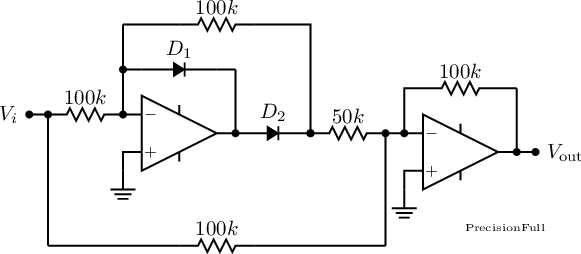
As a simple example, try a point-and-click solution to placing the bottom 100k resistor exactly centrally!
Yes, I still use xfig, I was one of the earlier users! It is still
one of the best CAD packages (for Unices, naturally :-) (2005 update: I
haven’t used it for 3 or 4 years now. I do EVERYTHING in Circuit
Macros/GNUpic)
The Circuit Macros are based on a mixture of the GNU m4 macro
language and the standard GNU pic language, and actually uses both.
The macro’s expand into pic—pic being one of the “little
languages” like eqn and tbl for pictures, equations and
tables which were extensions of troff, the original Unix Document
Typesetting language, written by a completely unknown author by the name of
Brian Kernighan, who wrote nothing else of Note, excepting the middle key
of the Piano.
As the figures are drawn using a powerful programming language, all standard programming features exist—the author has some stunning examples using for loops, subfunctions etc.
For plebs like me though, the macro’s are put together so well that the learning curve is particularly easy, without getting too fancy!
As a simple example of the use of a for loop, consider a simple
ground plane:
As an example of what can be done, I have processed all of my Electronics I (second year) lecture notes and present them by chapter. My Electromagnetics (third year), High Frequency Techniques (= Antennas) (fourth year) and several other miscellaneous things from various CPD courses that I run.
| Chapter 1 Op-Amps | Chapter 2 Digital Basics | Chapter 3 Diodes |
| Chapter 4 Bipolar Junction Transistors | Chapter 5 MOSFETS | Chapter 6 Applications |
For ELEN302, Electromagnetics, in the third year:
Likewise for HF Techniques (4th year elective course):
| Chapter 1 Antenna Fundamentals | Chapter 2 Thin Linear Antennas | Chapter 3 Array Theory |
| Chapter 4 Antenna Types |
Miscellaneous: Miscellaneous Figures
As root, change dir to "/usr/local" and unpack the archive there
using tar -zxf cm.tgz
Ensure that /usr/local/bin is in your path (It should be!!) for
the scripts cct, ccteg, cctgif.
Set an environment variable in ~/.bashrc with
export M4PATH=/usr/local/lib/cct
Check that m4 and gpic are installed (which).
You’re done.
Read the docs in the /usr/local/doc/cct (I have also included the
classic PIC manual by Brian Kernighan) (and converted them to pdf too, just
in case)
Since MsLoss has no sense of lib and bin, choose a suitable
installation directory, (eg /apps/cct) and unzip the archive. Move the
batch files cct.bat ccteg.bat cctgif.bat to somewhere on your path.
Set the environment variable M4PATH to wherever your libs are.
In the initial stages of laying out a new circuit (or any figure, I now use “Circuit Macros” for pretty much every graphical thing I need), it is useful to have an easy preview method. Since this entails a latex run, and I cannot pass a file name as a variable, I adopt a rigid filename. All new circuits are called ccteg.m4, and I use a little script ccteg to process it. I leave xdvi running in another screen so that it updates in real time. In the Dos world, similar batch files can be written. MikTeX provides YAP as the previewer, which can show the tpic specials.
I have made some minor modifications to the macros, allowing an additional parameter to a diode to denote an LED, modified the op-amp a tad, and added the power-supply connections—students simply don’t power these things up!!! Some of these have been adopted by the author of the macros. (I have reverted to using the original stuff now, as most “important” (to me) suggestions have been adopted by the original author!—try that with Uncle Bill :-)
I have also removed the hardcoded paths in ALL m4 files, and use M4PATH instead. ie I have changed: (in each file)
#ifdef(`HOMELIB_',,`define(`HOMELIB_',`/u/aplevich/lib/')')
ifdef(`HOMELIB_',,`define(`HOMELIB_',`')')
My convention of using .cct and \inputcct actually using the
tpic specials is now deprecated: a .cct file is not really shareable
with non-LATEX 2є users. (I could say something here, but I’ll be
good). So my new cct script produces (via an m4 run, a
gpic run, a LATEXrun, a dvips run, two gs runs,
within the netpbm suite, we have a call to
pnmcrop, pnmmargin, pnmalias, and pnmtopng. Finally a sed call sorts out the correct BoundingBox
in the Encapsulated Postscript. :-) an .eps file and a web-able
.png file. (Google
burnallgifs) This entire procedure is completely transparent to the user,
and from the original .m4 picture file, we magically simply get a
.eps and a .png in the same directory.
Naturally cct *.m4 processes all figures in the directory. Try that
in Doze :-)
The Encapsulated Postscript is inserted with \inputepsraw{fn}{cap}
available from my ftp
site, the snippet of interest (from the .dtx file) being:
\newcommand{\inputepsraw}[2]%
  {%
    \begin{figure}[!htb]%
      \centering%
      \includegraphics{#1.eps}%
      \caption{#2}%    includes fig num
      \label{fig:#1}%  ie may \ref{fig:#1}
    \end{figure}%
  }
Note that this includes the file at “natural” scaling, ie 10*mm in m4 will be 10mm on the printed page.
The relevant section from the cct.hva Hevea style file is:
% A replacement for \inputeps of the ArcMacro package, for the purpose of
% .png inclusion of the cct macros generated .eps, for Web use.
%
% Alan Robert Clark a.clark@ee.wits.ac.za
%
% created 10 March 2005.

\renewcommand{\inputepsraw}[3][80]%
  {% Dont use height in HeVeA, but keep interface the same :-)
    \begin{figure*}[!htb]%
        \centering%
 \ahref{cctpng/#2.txt}{%
          \imgsrc{cctpng/#2.png}%
 }
        \caption{#3}%    includes fig num
        \label{fig:#2}%  ie may \ref{fig:#2}
    \end{figure*}%
  }
dimen_. I tried
following the idea of absolute grids as in the author’s first example, but
this was not meant as general rule, and it becomes very tedious.This convention has also changed. Every new file automatically includes the following standard definitions:
# Usual defs...
qrt=dimen_/4;
hlf=dimen_/2;
dim=dimen_;
mm=1/25.4;
pi=atan2(0,-1);
This allows mm to be the default when drawing arb things, and dim, hlf, qrt when actually using Circuit Elements.
resistor (right_) instead of
resistor(right_) Its a pain, but you get used to it :-) (m4
Hangover, apparently)line to (Op1.Out, Here) line to (Here, Op1.Out)This is because both Here and Op1.Out have an x and a y component; in the first line, the x component of Op1.Out is used, and in the second line the y component.
# at the beggining of lines to comment
them out, until you find your glaring error!line right_ dimen_/2;dot
{line down_ dimen_/4;dot; "-10V" ljust_}
line right_ dimen_/2
where the third line takes off from where the first finished, not from
where the second finished.The scripts are
The online version is "http://ytdp.ee.wits.ac.za/cct.html"
This document was translated from LATEX by HEVEA.